Resampling of swath data
Pyresample can be used to resample a swath dataset to a grid, a grid to a swath or a swath to another swath. Resampling can be done using nearest neighbour method, Guassian weighting, weighting with an arbitrary radial function.
Changed in version 1.8.0: SwathDefinition no longer checks the validity of the provided longitude
and latitude coordinates to improve performance. Longitude arrays are
expected to be between -180 and 180 degrees, latitude -90 to 90 degrees.
This also applies to all geometry definitions that are provided longitude
and latitude arrays on initialization. Use
check_and_wrap() to preprocess your arrays.
pyresample.image
The ImageContainerNearest and ImageContanerBilinear classes can be used for resampling of swaths as well as grids. Below is an example using nearest neighbour resampling.
>>> import numpy as np
>>> from pyresample import image, geometry
>>> area_def = geometry.AreaDefinition('areaD', 'Europe (3km, HRV, VTC)', 'areaD',
...                                {'a': '6378144.0', 'b': '6356759.0',
...                                 'lat_0': '50.00', 'lat_ts': '50.00',
...                                 'lon_0': '8.00', 'proj': 'stere'},
...                                800, 800,
...                                [-1370912.72, -909968.64,
...                                 1029087.28, 1490031.36])
>>> data = np.fromfunction(lambda y, x: y*x, (50, 10))
>>> lons = np.fromfunction(lambda y, x: 3 + x, (50, 10))
>>> lats = np.fromfunction(lambda y, x: 75 - y, (50, 10))
>>> swath_def = geometry.SwathDefinition(lons=lons, lats=lats)
>>> swath_con = image.ImageContainerNearest(data, swath_def, radius_of_influence=5000)
>>> area_con = swath_con.resample(area_def)
>>> result = area_con.image_data
For other resampling types or splitting the process in two steps use e.g. the functions in pyresample.kd_tree described below.
pyresample.kd_tree
This module contains several functions for resampling swath data.
Note distance calculation is approximated with cartesian distance.
Masked arrays can be used as data input. In order to have undefined pixels masked out instead of assigned a fill value set fill_value=None when calling the resample_* function.
resample_nearest
Function for resampling using nearest neighbour method.
Example showing how to resample a generated swath dataset to a grid using nearest neighbour method:
>>> import numpy as np
>>> from pyresample import kd_tree, geometry
>>> area_def = geometry.AreaDefinition('areaD', 'Europe (3km, HRV, VTC)', 'areaD',
...                                {'a': '6378144.0', 'b': '6356759.0',
...                                 'lat_0': '50.00', 'lat_ts': '50.00',
...                                 'lon_0': '8.00', 'proj': 'stere'},
...                                800, 800,
...                                [-1370912.72, -909968.64,
...                                 1029087.28, 1490031.36])
>>> data = np.fromfunction(lambda y, x: y*x, (50, 10))
>>> lons = np.fromfunction(lambda y, x: 3 + x, (50, 10))
>>> lats = np.fromfunction(lambda y, x: 75 - y, (50, 10))
>>> swath_def = geometry.SwathDefinition(lons=lons, lats=lats)
>>> result = kd_tree.resample_nearest(swath_def, data,
... area_def, radius_of_influence=50000, epsilon=0.5)
If the arguments swath_def and area_def where switched (and data matched the dimensions of area_def) the grid of area_def would be resampled to the swath defined by swath_def.
Note the keyword arguments:
radius_of_influence: The radius around each grid pixel in meters to search for neighbours in the swath.
epsilon: The distance to a found value is guaranteed to be no further than (1 + eps) times the distance to the correct neighbour. Allowing for uncertanty decreases execution time.
If data is a masked array the mask will follow the neighbour pixel assignment.
If there are multiple channels in the dataset the data argument should be of the shape of the lons and lat arrays with the channels along the last axis e.g. (rows, cols, channels). Note: the convention of pyresample < 0.7.4 is to pass data in the form of (number_of_data_points, channels) is still accepted.
>>> import numpy as np
>>> from pyresample import kd_tree, geometry
>>> area_def = geometry.AreaDefinition('areaD', 'Europe (3km, HRV, VTC)', 'areaD',
...                                {'a': '6378144.0', 'b': '6356759.0',
...                                 'lat_0': '50.00', 'lat_ts': '50.00',
...                                 'lon_0': '8.00', 'proj': 'stere'},
...                                800, 800,
...                                [-1370912.72, -909968.64,
...                                 1029087.28, 1490031.36])
>>> channel1 = np.fromfunction(lambda y, x: y*x, (50, 10))
>>> channel2 = np.fromfunction(lambda y, x: y*x, (50, 10)) * 2
>>> channel3 = np.fromfunction(lambda y, x: y*x, (50, 10)) * 3
>>> data = np.dstack((channel1, channel2, channel3))
>>> lons = np.fromfunction(lambda y, x: 3 + x, (50, 10))
>>> lats = np.fromfunction(lambda y, x: 75 - y, (50, 10))
>>> swath_def = geometry.SwathDefinition(lons=lons, lats=lats)
>>> result = kd_tree.resample_nearest(swath_def, data,
... area_def, radius_of_influence=50000)
For nearest neighbour resampling the class image.ImageContainerNearest can be used as well as kd_tree.resample_nearest
resample_gauss
Function for resampling using nearest Gussian weighting. The Gauss weigh function is defined as exp(-dist^2/sigma^2). Note the pyresample sigma is not the standard deviation of the gaussian. Example showing how to resample a generated swath dataset to a grid using Gaussian weighting:
>>> import numpy as np
>>> from pyresample import kd_tree, geometry
>>> area_def = geometry.AreaDefinition('areaD', 'Europe (3km, HRV, VTC)', 'areaD',
...                                {'a': '6378144.0', 'b': '6356759.0',
...                                 'lat_0': '50.00', 'lat_ts': '50.00',
...                                 'lon_0': '8.00', 'proj': 'stere'},
...                                800, 800,
...                                [-1370912.72, -909968.64,
...                                 1029087.28, 1490031.36])
>>> data = np.fromfunction(lambda y, x: y*x, (50, 10))
>>> lons = np.fromfunction(lambda y, x: 3 + x, (50, 10))
>>> lats = np.fromfunction(lambda y, x: 75 - y, (50, 10))
>>> swath_def = geometry.SwathDefinition(lons=lons, lats=lats)
>>> result = kd_tree.resample_gauss(swath_def, data,
... area_def, radius_of_influence=50000, sigmas=25000)
If more channels are present in data the keyword argument sigmas must be a list containing a sigma for each channel.
If data is a masked array any pixel in the result data that has been “contaminated” by weighting of a masked pixel is masked.
Using the function utils.fwhm2sigma the sigma argument to the gauss resampling can be calculated from 3 dB FOV levels.
resample_custom
Function for resampling using arbitrary radial weight functions.
Example showing how to resample a generated swath dataset to a grid using an arbitrary radial weight function:
>>> import numpy as np
>>> from pyresample import kd_tree, geometry
>>> area_def = geometry.AreaDefinition('areaD', 'Europe (3km, HRV, VTC)', 'areaD',
...                                {'a': '6378144.0', 'b': '6356759.0',
...                                 'lat_0': '50.00', 'lat_ts': '50.00',
...                                 'lon_0': '8.00', 'proj': 'stere'},
...                                800, 800,
...                                [-1370912.72, -909968.64,
...                                 1029087.28, 1490031.36])
>>> data = np.fromfunction(lambda y, x: y*x, (50, 10))
>>> lons = np.fromfunction(lambda y, x: 3 + x, (50, 10))
>>> lats = np.fromfunction(lambda y, x: 75 - y, (50, 10))
>>> swath_def = geometry.SwathDefinition(lons=lons, lats=lats)
>>> wf = lambda r: 1 - r/100000.0
>>> result  = kd_tree.resample_custom(swath_def, data,
...  area_def, radius_of_influence=50000, weight_funcs=wf)
If more channels are present in data the keyword argument weight_funcs must be a list containing a radial function for each channel.
If data is a masked array any pixel in the result data that has been “contaminated” by weighting of a masked pixel is masked.
Uncertainty estimates
Uncertainty estimates in the form of weighted standard deviation can be obtained from the resample_custom and resample_gauss functions. By default the functions return the result of the resampling as a single numpy array. If the functions are given the keyword argument with_uncert=True then the following list of numpy arrays will be returned instead: (result, stddev, count). result is the usual result. stddev is the weighted standard deviation for each element in the result. count is the number of data values used in the weighting for each element in the result.
The principle is to view the calculated value for each element in the result as a weighted average of values sampled from a statistical variable. An estimate of the standard deviation of the distribution is calculated using the unbiased weighted estimator given as stddev = sqrt((V1 / (V1 ** 2 + V2)) * sum(wi * (xi - result) ** 2)) where result is the result of the resampling. xi is the value of a contributing neighbour and wi is the corresponding weight. The coefficients are given as V1 = sum(wi) and V2 = sum(wi ** 2). The standard deviation is only calculated for elements in the result where more than one neighbour has contributed to the weighting. The count numpy array can be used for filtering at a higher number of contributing neigbours.
Usage only differs in the number of return values from resample_gauss and resample_custom. E.g.:
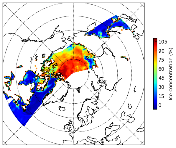
>>> result, stddev, count = pr.kd_tree.resample_gauss(swath_def, ice_conc, area_def,
...                                                   radius_of_influence=20000,
...                                                   sigmas=pr.utils.fwhm2sigma(35000),
...                                                   fill_value=None, with_uncert=True)
- Below is shown a plot of the result of the resampling using a real data set:
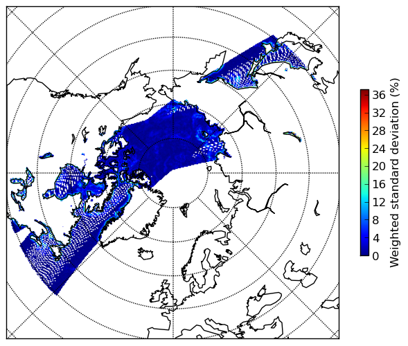
- The corresponding standard deviations:
- And the number of contributing neighbours for each element:
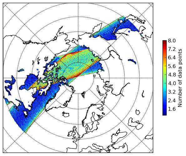
Notice the standard deviation is only calculated where there are more than one contributing neighbour.
Resampling from neighbour info
The resampling can be split in two steps:
First get arrays containing information about the nearest neighbours to each grid point. Then use these arrays to retrive the resampling result.
This approch can be useful if several datasets based on the same swath are to be resampled. The computational heavy task of calculating the neighbour information can be done once and the result can be used to retrieve the resampled data from each of the datasets fast.
>>> import numpy as np
>>> from pyresample import kd_tree, geometry
>>> area_def = geometry.AreaDefinition('areaD', 'Europe (3km, HRV, VTC)', 'areaD',
...                                {'a': '6378144.0', 'b': '6356759.0',
...                                 'lat_0': '50.00', 'lat_ts': '50.00',
...                                 'lon_0': '8.00', 'proj': 'stere'},
...                                800, 800,
...                                [-1370912.72, -909968.64,
...                                 1029087.28, 1490031.36])
>>> data = np.fromfunction(lambda y, x: y*x, (50, 10))
>>> lons = np.fromfunction(lambda y, x: 3 + x, (50, 10))
>>> lats = np.fromfunction(lambda y, x: 75 - y, (50, 10))
>>> swath_def = geometry.SwathDefinition(lons=lons, lats=lats)
>>> valid_input_index, valid_output_index, index_array, distance_array = \
...                        kd_tree.get_neighbour_info(swath_def,
...                                                       area_def, 50000,
...                                                   neighbours=1)
>>> res = kd_tree.get_sample_from_neighbour_info('nn', area_def.shape, data,
...                                              valid_input_index, valid_output_index,
...                                              index_array)
Note the keyword argument neighbours=1. This specifies only to consider one neighbour for each grid point (the nearest neighbour). Also note distance_array is not a required argument for get_sample_from_neighbour_info when using nearest neighbour resampling
Segmented resampling
Whenever a resampling function takes the keyword argument segments the number of segments to split the resampling process in can be specified. This affects the memory footprint of pyresample. If the value of segments is left to default pyresample will estimate the number of segments to use.
pyresample.bilinear
Compared to nearest neighbour resampling, bilinear interpolation produces smoother results near swath edges of polar satellite data and edges of geostationary satellites.
The algorithm is implemented from http://www.ahinson.com/algorithms_general/Sections/InterpolationRegression/InterpolationIrregularBilinear.pdf
Below is shown a comparison between image generated with nearest neighbour resampling (top) and with bilinear interpolation (bottom):
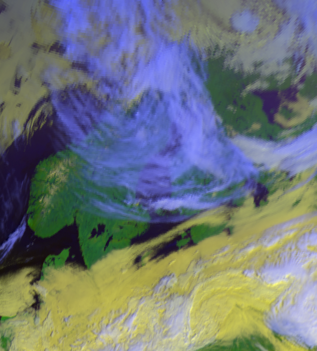

Click images to see the full resolution versions.
The perceived sharpness of the bottom image is lower, but there is more detail present.
XArrayBilinearResampler
bilinear.XArrayBilinearResampler is a class that handles bilinear interpolation for data in xarray.DataArray arrays. The parallelization is done automatically using dask.
>>> import numpy as np
>>> import dask.array as da
>>> from xarray import DataArray
>>> from pyresample.bilinear import XArrayBilinearResampler
>>> from pyresample import geometry
>>> target_def = geometry.AreaDefinition('areaD',
...                                      'Europe (3km, HRV, VTC)',
...                                      'areaD',
...                                      {'a': '6378144.0', 'b': '6356759.0',
...                                       'lat_0': '50.00', 'lat_ts': '50.00',
...                                       'lon_0': '8.00', 'proj': 'stere'},
...                                      800, 800,
...                                      [-1370912.72, -909968.64,
...                                       1029087.28, 1490031.36])
>>> data = DataArray(da.from_array(np.fromfunction(lambda y, x: y*x, (500, 100))), dims=('y', 'x'))
>>> lons = da.from_array(np.fromfunction(lambda y, x: 3 + x * 0.1, (500, 100)))
>>> lats = da.from_array(np.fromfunction(lambda y, x: 75 - y * 0.1, (500, 100)))
>>> source_def = geometry.SwathDefinition(lons=lons, lats=lats)
>>> resampler = XArrayBilinearResampler(source_def, target_def, 30e3)
>>> result = resampler.resample(data)
The resampling info can be saved for later reuse and much faster processing for a matching area. The data are saved to a Zarr archive, so zarr Python package needs to be installed.
>>> import os
>>> from tempfile import gettempdir
>>> cache_file = os.path.join(gettempdir(), "bilinear_resampling_luts.zarr")
>>> resampler.save_resampling_info(cache_file)
>>> new_resampler = XArrayBilinearResampler(source_def, target_def, 30e3)
>>> new_resampler.load_resampling_info(cache_file)
>>> result = new_resampler.resample(data)
NumpyBilinearResampler
bilinear.NumpyBilinearResampler is a plain Numpy version of XArrayBilinearResampler. If fill_value isn’t given to get_sample_from_bil_info(), a masked array will be returned.
>>> import numpy as np
>>> from pyresample.bilinear import NumpyBilinearResampler
>>> from pyresample import geometry
>>> target_def = geometry.AreaDefinition('areaD',
...                                      'Europe (3km, HRV, VTC)',
...                                      'areaD',
...                                      {'a': '6378144.0', 'b': '6356759.0',
...                                       'lat_0': '50.00', 'lat_ts': '50.00',
...                                       'lon_0': '8.00', 'proj': 'stere'},
...                                      800, 800,
...                                      [-1370912.72, -909968.64,
...                                       1029087.28, 1490031.36])
>>> data = np.fromfunction(lambda y, x: y*x, (500, 100))
>>> lons = np.fromfunction(lambda y, x: 3 + x * 0.1, (500, 100))
>>> lats = np.fromfunction(lambda y, x: 75 - y * 0.1, (500, 100))
>>> source_def = geometry.SwathDefinition(lons=lons, lats=lats)
>>> resampler = NumpyBilinearResampler(source_def, target_def, 30e3)
>>> result = resampler.resample(data)
resample_bilinear
Convenience function for resampling using bilinear interpolation for irregular source grids.
Note
The use of this function is deprecated. Depending on the input data format, please use directly the bilinear.NumpyBilinearResampler or bilinear.XArrayBilinearResampler classes and their .resample() method shown above.
>>> import numpy as np
>>> from pyresample import bilinear, geometry
>>> target_def = geometry.AreaDefinition('areaD',
...                                      'Europe (3km, HRV, VTC)',
...                                      'areaD',
...                                      {'a': '6378144.0', 'b': '6356759.0',
...                                       'lat_0': '50.00', 'lat_ts': '50.00',
...                                       'lon_0': '8.00', 'proj': 'stere'},
...                                      800, 800,
...                                      [-1370912.72, -909968.64,
...                                       1029087.28, 1490031.36])
>>> data = np.fromfunction(lambda y, x: y*x, (500, 100))
>>> lons = np.fromfunction(lambda y, x: 3 + x * 0.1, (500, 100))
>>> lats = np.fromfunction(lambda y, x: 75 - y * 0.1, (500, 100))
>>> source_def = geometry.SwathDefinition(lons=lons, lats=lats)
>>> result = bilinear.resample_bilinear(data, source_def, target_def,
...                                     radius=50e3, neighbours=32,
...                                     nprocs=1, fill_value=0,
...                                     reduce_data=True, segments=None,
...                                     epsilon=0)
The target_area needs to be an area definition with proj_str attribute.
Keyword arguments which are passed to kd_tree:
radius: radius around each target pixel in meters to search for neighbours in the source data
neighbours: number of closest locations to consider when selecting the four data points around the target location. Note that this value needs to be large enough to ensure “surrounding” the target!
nprocs: number of processors to use for finding the closest pixels
fill_value: fill invalid pixel with this value. If fill_value=None is used, masked arrays will be returned
reduce_data: do/don’t do preliminary data reduction before calculating the neigbour info
epsilon: maximum uncertainty allowed in neighbour search
The example above shows the default value for each keyword argument.
Resampling from bilinear coefficients
Note
This usage is deprecated, please use the bilinear.NumpyBilinearResampler or bilinear.XArrayBilinearResampler classes directly depending on the input data format.
As for nearest neighbour resampling, also bilinear interpolation can be split in two steps.
Calculate interpolation coefficients, input data reduction matrix and mapping matrix
Use this information to resample several datasets between these two areas/swaths
Only the first step is computationally expensive operation, so by re-using this information the overall processing time is reduced significantly. This is also done internally by the resample_bilinear function, but separating these steps makes it possible to cache the coefficients if the same transformation is done over and over again. This is very typical in operational geostationary satellite image processing. Note that the output shape is now defined so that the result is reshaped to correct shape. This reshaping is done internally in resample_bilinear.
>>> import numpy as np
>>> from pyresample import bilinear, geometry
>>> target_def = geometry.AreaDefinition('areaD', 'Europe (3km, HRV, VTC)',
...                                      'areaD',
...                                      {'a': '6378144.0', 'b': '6356759.0',
...                                       'lat_0': '50.00', 'lat_ts': '50.00',
...                                       'lon_0': '8.00', 'proj': 'stere'},
...                                      800, 800,
...                                      [-1370912.72, -909968.64,
...                                       1029087.28, 1490031.36])
>>> data = np.fromfunction(lambda y, x: y*x, (50, 10))
>>> lons = np.fromfunction(lambda y, x: 3 + x, (50, 10))
>>> lats = np.fromfunction(lambda y, x: 75 - y, (50, 10))
>>> source_def = geometry.SwathDefinition(lons=lons, lats=lats)
>>> t_params, s_params, input_idxs, idx_ref = \
...     bilinear.get_bil_info(source_def, target_def, radius=50e3, nprocs=1)
>>> res = bilinear.get_sample_from_bil_info(data.ravel(), t_params, s_params,
...                                         input_idxs, idx_ref,
...                                         output_shape=target_def.shape)
pyresample.ewa
Pyresample makes it possible to resample swath data to a uniform grid using an Elliptical Weighted Averaging algorithm or EWA for short. This algorithm behaves differently than the KDTree based resampling algorithms that pyresample provides. The KDTree-based algorithms process each output grid pixel by searching for all “nearby” input pixels and applying a certain interpolation (nearest neighbor, gaussian, etc). The EWA algorithm processes each input pixel mapping it to one or more output pixels. Once each input pixel has been analyzed, the intermediate results are averaged to produce the final gridded result.
The EWA algorithm also has limitations on how the input data are structured
compared to the generic KDTree algorithms. EWA assumes that data in the array
is organized geographically; adjacent data in the array is adjacent data
geographically. The algorithm uses this to configure parameters based on the
size and location of the swath pixels. It also assumes that data are
scan-based, recorded by a orbiting satellite scan by scan, and the user must
provide scan size with the rows_per_scan option.
The EWA algorithm consists of two steps: ll2cr and fornav. The algorithm was originally part of the MODIS Swath to Grid Toolbox (ms2gt) created by the NASA National Snow & Ice Data Center (NSIDC). Its default parameters work best with MODIS L1B data, but it has been proven to produce high quality images from VIIRS and AVHRR data with the right parameters.
Note
This code was originally part of the CSPP Polar2Grid project. This documentation and the API documentation for this algorithm may still use references or concepts from Polar2Grid until everything can be updated.
Resampler
The DaskEWAResampler is the easiest way to use the
EWA resampling algorithm. Internally this resampler uses the dask library
to perform all of its operations in parallel. This will typically provide
better performance than any of the below methods, but does require the
dask library to be installed. The below code assumes you have a
swath_def object (SwathDefinition), an
area_def object (AreaDefinition), and
some array data in data. Data can be a numpy array, a dask array, or
an xarray DataArray object.
from pyresample.ewa import DaskEWAResampler
resampler = DaskEWAResampler(swath_def, area_def)

# if the data are scan based, specify how many data rows make up one scan
rows_per_scan = 5
result = resampler.resample(data, rows_per_scan=rows_per_scan)
Note
As a convenience, you can set rows_per_scan to 0 to have it set to the number of rows in the input data. This can be helpful when testing EWA on data that is not necessarily scan based, but still has nice results with EWA.
Legacy Dask Resampler
This resampler is similar to the above, but only works on xarray DataArray objects backed by dask arrays. Although it uses dask underneath, it doesn’t use it optimally and in most cases will use a lot of memory.
from pyresample.ewa import LegacyDaskEWAResampler
resampler = LegacyDaskEWAResampler(xr_swath_def, area_def)

# if the data are scan based, specify how many data rows make up one scan
rows_per_scan = 5
result = resampler.resample(xr_data, rows_per_scan=rows_per_scan)
Legacy Function Interface
It is recommended to use the Resampler interfaces described above whenever
possible. However, the low-level ll2cr and fornav functions can be
used if desired. These functions will only work on basic numpy arrays and
although fast, they will use a lot of memory for large input arrays or large
target areas.
from pyresample.ewa import ll2cr, fornav
# ll2cr converts swath longitudes and latitudes to grid columns and rows
swath_points_in_grid, cols, rows = ll2cr(swath_def, area_def)
# if the data are scan based, specify how many data rows make up one scan
rows_per_scan = 5
# fornav resamples the swath data to the gridded area
num_valid_points, gridded_data = fornav(cols, rows, area_def, data, rows_per_scan=rows_per_scan)
pyresample.bucket
- class pyresample.bucket.BucketResampler(target_area, source_lons, source_lats)
Bucket resampler.
Bucket resampling is useful for calculating averages and hit-counts when aggregating data to coarser scale grids.
Below are examples how to use the resampler.
Read data using Satpy. The resampling can also be done (apart from fractions) directly from Satpy, but this demonstrates the direct low-level usage.
>>> from pyresample.bucket import BucketResampler
>>> from satpy import Scene
>>> from satpy.resample import get_area_def
>>> fname = "hrpt_noaa19_20170519_1214_42635.l1b"
>>> glbl = Scene(filenames=[fname])
>>> glbl.load(['4'])
>>> data = glbl['4']
>>> lons, lats = data.area.get_lonlats()
>>> target_area = get_area_def('euro4')
Initialize the resampler
>>> resampler = BucketResampler(target_area, lons, lats)
Calculate the sum of all the data in each grid location:
>>> sums = resampler.get_sum(data)
Calculate how many values were collected at each grid location:
>>> counts = resampler.get_count()
The average can be calculated from the above two results, or directly using the helper method:
>>> average = resampler.get_average(data)
Calculate fractions of occurrences of different values in each grid location. The data needs to be categorical (in integers), so we’ll create some categorical data from the brightness temperature data that were read earlier. The data are returned in a dictionary with the categories as keys.
>>> data = da.where(data > 250, 1, 0)
>>> fractions = resampler.get_fractions(data, categories=[0, 1])
>>> import matplotlib.pyplot as plt
>>> plt.imshow(fractions[0]); plt.show()
- __init__(target_area, source_lons, source_lats)
- __reduce_ex__(protocol, /)
Helper for pickle.
See BucketResampler API documentation for
the details of method parameters.