Plotting with pyresample and Cartopy
Pyresample supports basic integration with Cartopy.
Displaying data quickly
Pyresample has some convenience functions for displaying data from a single
channel. The show_quicklook function
shows a Cartopy generated image of a dataset for a specified AreaDefinition.
The function save_quicklook saves the Cartopy image directly to file.
Example usage:
In this simple example below we use GCOM-W1 AMSR-2 data loaded using Satpy. Satpy simplifies the reading of this data, but is not necessary for using pyresample or plotting data.
First we read in the data with Satpy:
>>> from satpy.scene import Scene
>>> from glob import glob
>>> SCENE_FILES = glob("./GW1AM2_20191122????_156*h5")
>>> scn = Scene(reader='amsr2_l1b', filenames=SCENE_FILES)
>>> scn.load(["btemp_36.5v"])
>>> lons, lats = scn["btemp_36.5v"].area.get_lonlats()
>>> tb37v = scn["btemp_36.5v"].data.compute()
Data for this example can be downloaded from zenodo.
If you have your own data, or just want to see that the example code here runs, you can
set the three arrays lons, lats and tb37v accordingly, e.g.:
>>> from pyresample.geometry import AreaDefinition
>>> area_id = 'ease_sh'
>>> description = 'Antarctic EASE grid'
>>> proj_id = 'ease_sh'
>>> projection = {'proj': 'laea', 'lat_0': -90, 'lon_0': 0, 'a': 6371228.0, 'units': 'm'}
>>> width = 425
>>> height = 425
>>> area_extent = (-5326849.0625, -5326849.0625, 5326849.0625, 5326849.0625)
>>> area_def = AreaDefinition(area_id, description, proj_id, projection,
...                           width, height, area_extent)
But here we go on with the loaded AMSR-2 data. Make sure you have an areas.yaml
file that defines the ease_sh area, or see
the area definition section on how to define one.
>>> from pyresample import load_area, save_quicklook, SwathDefinition
>>> from pyresample.kd_tree import resample_nearest
>>> swath_def = SwathDefinition(lons, lats)
>>> result = resample_nearest(swath_def, tb37v, area_def,
...                           radius_of_influence=20000, fill_value=None)
>>> save_quicklook('tb37v_quick.png', area_def, result, label='Tb 37v (K)')
Assuming lons, lats and tb37v are initialized with real data (as in the above Satpy example) the result might look something like this:
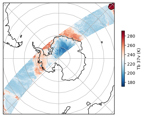
The data passed to the functions is a 2D array matching the AreaDefinition.
The Plate Carree projection
The Plate Carree projection (regular lon/lat grid) is named eqc in Proj.4. Pyresample uses the Proj.4 naming.
Assuming the file areas.yaml has the following area definition:
pc_world:
  description: Plate Carree world map
  projection:
    proj: eqc
    ellps: WGS84
  shape:
    height: 480
    width: 640
  area_extent:
    lower_left_xy: [-20037508.34, -10018754.17]
    upper_right_xy: [20037508.34, 10018754.17]
Example usage:
>>> import matplotlib.pyplot as plt
>>> from pyresample import load_area, save_quicklook
>>> from pyresample.kd_tree import resample_nearest
>>> area_def = load_area('areas.yaml', 'pc_world')
>>> result = resample_nearest(swath_def, tb37v, area_def, radius_of_influence=20000, fill_value=None)
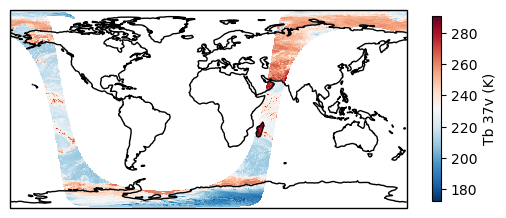
>>> save_quicklook('tb37v_pc.png', area_def, result, num_meridians=None, num_parallels=None, label='Tb 37v (K)')
Assuming lons, lats and tb37v are initialized with real data (like above we use AMSR-2 data in this example) the result might look something like this:
The Globe projections
From v0.7.12 pyresample can use the geos, ortho and nsper projections with Basemap. Starting with v1.9.0 quicklooks are now generated with Cartopy which should also work with these projections. Again assuming the area-config file areas.yaml has the following definition for an ortho projection area:
ortho:
  description: Ortho globe
  projection:
    proj: ortho
    lon_0: 40.
    lat_0: -40.
    a: 6370997.0
  shape:
    height: 480
    width: 640
  area_extent:
    lower_left_xy: [-10000000, -10000000]
    upper_right_xy: [10000000, 10000000]
Example usage:
>>> from pyresample import load_area, save_quicklook, SwathDefinition
>>> from pyresample.kd_tree import resample_nearest
>>> from pyresample import load_area
>>> area_def = load_area('areas.yaml', 'ortho')
>>> swath_def = SwathDefinition(lons, lats)
>>> result = resample_nearest(swath_def, tb37v, area_def, radius_of_influence=20000, fill_value=None)
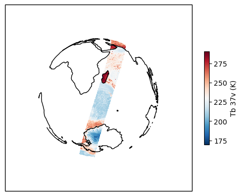
>>> save_quicklook('tb37v_ortho.png', area_def, result, num_meridians=None, num_parallels=None, label='Tb 37v (K)')
Assuming lons, lats and tb37v are initialized with real data, like in the above examples, the result might look something like this:
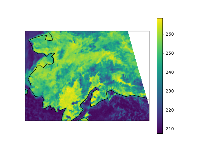
Getting a Cartopy CRS
To make more advanced plots than the preconfigured quicklooks Cartopy can be used to work with mapped data alongside matplotlib. The below code is based on this Cartopy gallery example. Pyresample allows any AreaDefinition to be converted to a Cartopy CRS as long as Cartopy can represent the projection. Once an AreaDefinition is converted to a CRS object it can be used like any other Cartopy CRS object.
>>> import matplotlib.pyplot as plt
>>> from pyresample.kd_tree import resample_nearest
>>> from pyresample.geometry import AreaDefinition
>>> area_id = 'alaska'
>>> description = 'Alaska Lambert Equal Area grid'
>>> proj_id = 'alaska'
>>> projection = {'proj': 'stere', 'lat_0': 62., 'lon_0': -152.5, 'ellps': 'WGS84', 'units': 'm'}
>>> width = 2019
>>> height = 1463
>>> area_extent = (-757214.993104, -485904.321517, 757214.993104, 611533.818622)
>>> area_def = AreaDefinition(area_id, description, proj_id, projection,
...                           width, height, area_extent)
>>> result = resample_nearest(swath_def, tb37v, area_def, radius_of_influence=20000, fill_value=None)
>>> crs = area_def.to_cartopy_crs()
>>> fig, ax = plt.subplots(subplot_kw=dict(projection=crs))
>>> coastlines = ax.coastlines()
>>> ax.set_global()
>>> img = plt.imshow(result, transform=crs, extent=crs.bounds, origin='upper')
>>> cbar = plt.colorbar()
>>> fig.savefig('amsr2_tb37v_cartopy.png')
Assuming lons, lats, and i04_data are initialized with real data the result might look something like this:
Getting a Basemap object
Warning
Basemap is no longer maintained. Cartopy (see above) should be used instead. Basemap does not support Matplotlib 3.0+ either.
In order to make more advanced plots than the preconfigured quicklooks a Basemap object can be generated from an
AreaDefinition using the area_def2basemap function.
Example usage:
>>> import matplotlib.pyplot as plt
>>> from pyresample.kd_tree import resample_nearest
>>> from pyresample.geometry import AreaDefinition
>>> area_id = 'ease_sh'
>>> description = 'Antarctic EASE grid'
>>> proj_id = 'ease_sh'
>>> projection = {'proj': 'laea', 'lat_0': -90, 'lon_0': 0, 'a': 6371228.0, 'units': 'm'}
>>> width = 425
>>> height = 425
>>> area_extent = (-5326849.0625, -5326849.0625, 5326849.0625, 5326849.0625)
>>> area_def = AreaDefinition(area_id, description, proj_id, projection,
...                           width, height, area_extent)
>>> from pyresample import area_def2basemap
>>> result = resample_nearest(swath_def, tb37v, area_def,
...                           radius_of_influence=20000, fill_value=None)
>>> bmap = area_def2basemap(area_def)
>>> bmng = bmap.bluemarble()
>>> col = bmap.imshow(result, origin='upper', cmap='RdBu_r')
>>> plt.savefig('tb37v_bmng.png', bbox_inches='tight')
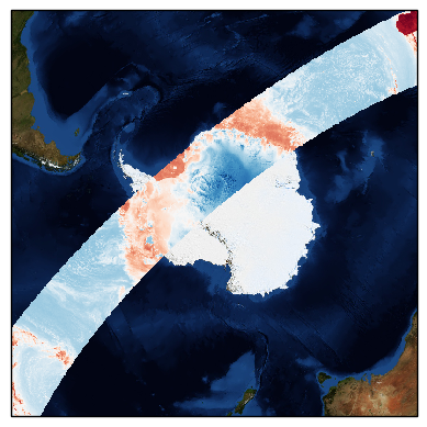
Assuming lons, lats and tb37v are initialized with real data as in the previous examples the result might look something like this:
Any keyword arguments (not concerning the projection) passed to plot.area_def2basemap will be passed directly to the Basemap initialization.
For more information on how to plot with Basemap please refer to the Basemap and matplotlib documentation.
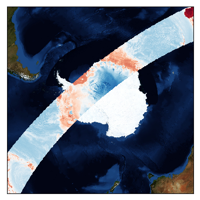
Adding background maps with Cartopy
As mentioned in the above warning Cartopy should be used rather than Basemap as the latter is not maintained anymore.
The above image can be generated using Cartopy instead by utilizing the method to_cartopy_crs of the AreaDefinition object.
Example usage:
>>> from pyresample.kd_tree import resample_nearest
>>> import matplotlib.pyplot as plt
>>> result = resample_nearest(swath_def, tb37v, area_def,
...                           radius_of_influence=20000, fill_value=None)
>>> crs = area_def.to_cartopy_crs()
>>> ax = plt.axes(projection=crs)
>>> ax.background_img(name='BM')
>>> plt.imshow(result, transform=crs, extent=crs.bounds, origin='upper', cmap='RdBu_r')
>>> plt.savefig('tb37v_bmng.png', bbox_inches='tight')
The above provides you have the Bluemarble background data available in the Cartopy standard place or in a directory pointed to by the environment parameter CARTOPY_USER_BACKGROUNDS.
With real data (same AMSR-2 as above) this might look like this: